Economic Order Quantity (EOQ)

A formula used in inventory strategy to determine the optimal order quantity that minimizes total inventory costs, including holding costs and ordering costs.

When is This Applicable?

This model is applicable when you have:

1. a variable inventory carrying cost. That is, there is a direct link to how many inventory you’re carrying and the cost to hold onto that.
2. a fixed cost to place an order, regardless of the order size. That is, there is a direct link to how many orders you place and the cost to place those orders.

Human Explanation

In reality, we use EOQ every day. Think about this simple case, you’re on a hike and have a water bottle. You can either stop to fill up your water bottle (lowkey tiring af) or you can keep walking but risk running out of water. At the same time, if you do stop to fill your water bottle, you’re going to have to carry that water around (highkey tiring af). So now you need to find a balance, how often should you fill your water bottle, and should you fill it all the way or only half way?

EOQ is a formula that helps you find that balance. It gives you the optimal order quantity that minimizes the total cost of inventory, which includes both the cost of holding inventory and the cost of placing orders.

Level 1: Constant Demand, No Lead Time

Assumptions:

• There is constant predictable demand
• There is no lead time, as soon as we place the order, we get the order

First, let’s look at the optimal model. The optimal looks something like a sawtooth, where we’re buying a bunch of inventory, then holding it until it runs out, then buying it again. This framework minimizes the total amount of inventory we hold onto, while also minimizing the number of orders we place.

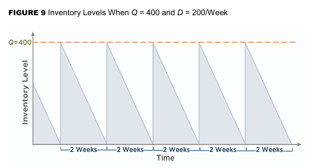
But now we must decide, how big should the sawtooths be?

Let’s define some variables:

• $D$ = demand (units per year)
• $K$ = ordering cost (cost per order)
• $h$ = holding cost (cost per unit per year)

Then, we can calculate the total cost of inventory as follows:

$$\text{Total Cost}=\text{Ordering Cost}+\text{Holding Cost}=\frac{D}{Q}K+\frac{Q}{2}h$$

This graph looks a bit like

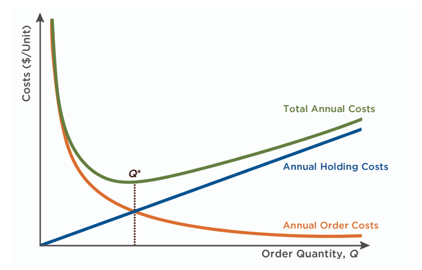
Using a simple first-order derivative we can compute the optimal order quantity $Q^{\ast }$ to be:

$$Q^{\ast }=\sqrt{\frac{2DK}{h}}$$

EZPZ!!

Level 2: Constant Demand, Lead Time

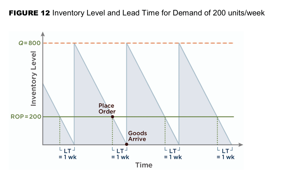
But what is there’s lead time? Let’s say, it takes two weeks between when we place an order and when we receive that order. In that case, we need to make sure we have enough inventory to meet demand during those two weeks.

This is easy, we simply place the order two weeks in advance. So, if we know our demand is 100 units per week, then we need to make sure we have at least 200 units of inventory on hand at all times to meet demand during the lead time.

So, we should define a “Reorder Point” (ROP), which is the inventory level at which we should place an order. The ROP can be calculated as follows:

$$ROP=dL$$

Where:

• $d$ = demand (units per week)
• $L$ = lead time (weeks)

Level 3: Variable Demand, Lead Time

Uh oh! Demand is squiggly now! What do we do, what if we run out during the lead time, it’s over…

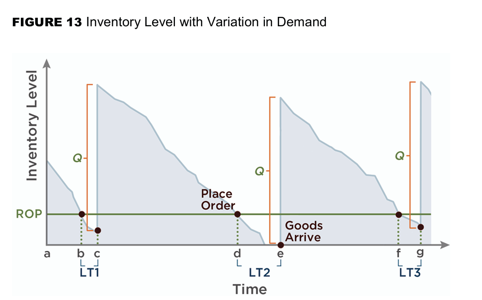
Here, our solution is to add safety stock, which is extra inventory we hold onto to protect against variability in demand and lead time. If demand is a normal distribution, it’s impossible to guarantee we won’t run out of inventory. The best we can do is to calculate the probability of running out of inventory and then decide how much safety stock to hold onto based on our risk tolerance.

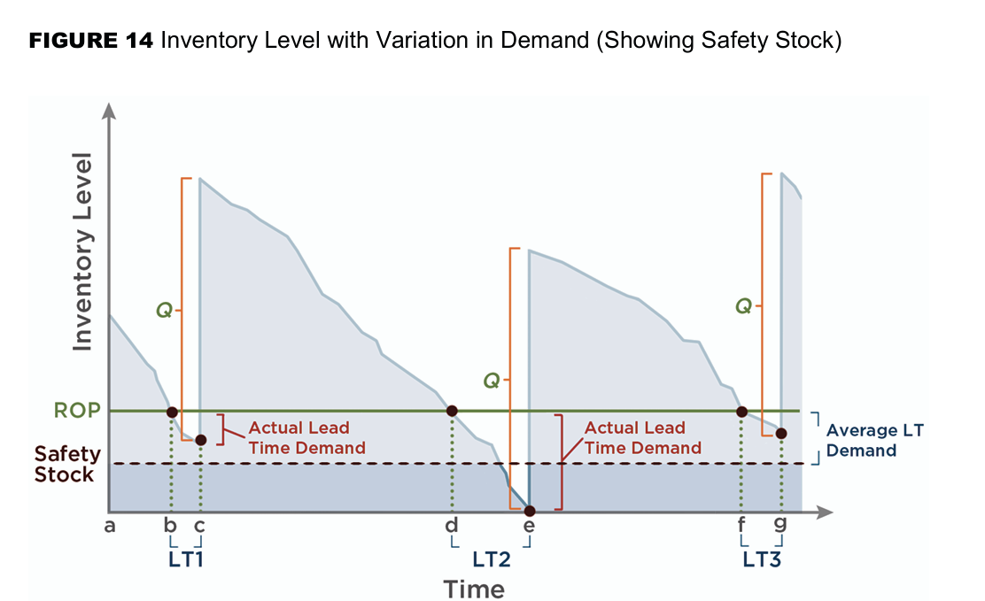
Now, ROP is calculated as follows:

$$ROP=dL+z{\sigma }_{dL}$$

or rather, ROP is the sum of the expected demand during the lead time, and our safety stock, which is a multiple $z$ of the standard deviation of demand during the lead time ${\sigma }_{dL}$.

$z$ here is the number of standard deviations we want to hold as safety stock, which is based on our desired service level. For example, if we want a 95% service level, we would look up the z-score for 95%, which is 1.65, and then multiply that by the standard deviation of demand during the lead time to get our safety stock.

Often times, we’re only giving the standard deviation of the demand per week ${\sigma }_d$, in which case we can calculate the standard deviation of demand during the lead time as follows:

$${\sigma }_{dL}={\sigma }_d\sqrt{L}$$

Giving us a final formal for ROP as

$$ROP=dL+z{\sigma }_d\sqrt{L}$$

Where:

• $d$ = demand (units per week)
• $L$ = lead time (weeks)
• $z$ = z-score corresponding to desired service level
• ${\sigma }_d$ = standard deviation of demand per week

Level 4: Periodic Review

Previously, we reordered when our inventory hits a certain point (i.e. ROP). However, this is not always possible. It’s not always possible to know your inventory level at every second or every day. Or rather, it might not be possible for you to reorder at any point. Maybe your supplier only accepts orders on Mondays. In that case, you need to switch to a periodic review system, where you review your inventory level at fixed intervals (e.g. every Monday) and then decide how much to order based on your inventory level at that time.

In our human analogy above, this would basically be, you don’t come across a water fountain all the time. Maybe there’s one every 250m

Our solution is, we will periodically check current inventory levels and place an order for the amount that will bring us up to a specified target level. Because of this, these systems are also called order-up-to systems.

The equivalent to this would be, I will fill my water bottle until it’s full when I come across a water fountain, regardless of my current water level.

Here our order quantity is:

$$\text{Order quantity}=\text{Expected demand during order interval}+\text{Expected demand during lead time}+\text{Safety stock}-\text{Current inventory level}$$